Learning data distribution involves identifying ‘key factors’, which inherently ‘control’ the characteristics of our observations. The controlling relationship can either be statistical, or based on physical laws, where we understand precisely how these factors manifest in data. We discuss these ‘key factors’, commonly referred to as latent variables, in detail below. First, we discuss their estimation from data using Variational Inference (VI). Then, we describe the opposite direction - data reconstruction and generation from latent variables.
Latent Space
Diffusion models are latent variable models (Ho et al., 2020; page 2). It is not only true when diffusion happens in the latent space of a Variational Autoencoder (for instance, in the Latent Diffusion case (Rombach et al., 2022)) but in general for Denoising Diffusion Probabilistic models. Let’s denote our training (or observed) data as \(\mathbf{x}_0\) (in Figure 1 in the Introduction chapter those would be noise-free cute ca… sorry… schematic Swiss-roll images at \(t=0\)) and its noised versions as \(\mathbf{z}_t\) with \(t=1:T\). In particular, \(\mathbf{z}_t\) corresponds to inputs \(\mathbf{x}_0\) with added noise, which comes from \(t\) Brownian jumps (see the full notation list in Appendix A). These noised versions make up the latent space of a diffusion model (Ho et al., 2020; page 2). Some authors instead of \(\mathbf{z}_t\) use \(\mathbf{x}_t\) to highlight a connection with input, but here we highlight \(\mathbf{z}_t\) being a latent space variable. We further call a sequence of latent spaces, or noised images, \(\mathbf{z}=(\mathbf{z}_1,\mathbf{z}_2,...,\mathbf{z}_T)\) an hierarchy. But for now, without the loss of generality, let’s abstract from a particular form of the latent space and “simply” denote it \(\mathbf{z}\).
What is a latent space? I, personally, really like the explanation provided in this video - MIT 6.S191: Deep Generative Modeling (7:53 time stamp). The analogy for latent space variables would be true objects (or true hidden factors), which cast shadows on the wall (or describe a physical process, which we register with some sort of sensors; Figure 1). In this case, the shadows would correspond to our observed data. Typically, latent variable would have less dimensions than the data we would like to describe. If we can estimate latent variables, we then can model complex distributions of observed data samples: if you know the object, you can predict its shadow.
Latent Variables are unobserved lower dimensional representations of higher dimensional inputs. They can be thought of as underlying factors responsible for the physical phenomenon we observe. For instance, the intensity of an earthquake at a particular location depends on such factors as: 1) the distance from the hypocenter 2) the ground you are at and 3) how large was the original displacement (not a full list). In machine learning, however, physical meaning of latents is not rigid but rather speculative and is subject to interpretation.
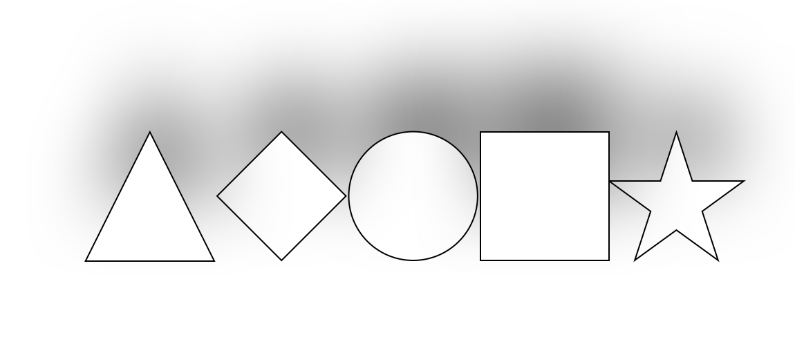 Figure 1: If you know true object shapes (latent variables) you can predict its shadows (observed data).
Variational Inference
To have an effective image generator, we need to find “true hidden” factors describing a variety of Swiss-roll schematics \(\mathbf{x}_0\) we have in our possession. We have a state of our hidden factors \(\mathbf{z}\) before and after seeing the data. Before, latent space \(\mathbf{z}\) naturally does not incorporate any knowledge about \(\mathbf{x}_0\). After seeing the data and estimating the latents, we hope \(\mathbf{z}\) becomes a lower-dimensional compressed representation of data. Besides searching for hidden factors, we can also search for the model, i.e., equation/precise law of physics/approximate relationship based on correlation/regression, which connects them to observations.
Formally, to obtain the latents and the model, the problem is posed in a Bayesian inference framework (Blei et al., 2018: page 2):
\[\begin{align} p(\mathbf{z},\mathbf{x}_0) = p(\mathbf{z})p(\mathbf{x}|\mathbf{z}) \end{align}\]So what do we actually see here? \(p\) stands for probability and \(p(\mathbf{z},\mathbf{x}_0)\) is joint probability density between latents and observed data. Physically, the latter describes how likely a certain combination of latents and observables can occur. A Bayesian model draws samples from the prior \(p(\mathbf{z})\) and then relates them to the observations through the likelihood \(p(\mathbf{x}_{0} | \mathbf{z})\) (Blei et al., 2018: page 2): the probability density of \(\mathbf{x}_0\) given a particular set of \(\mathbf{z}\). Imagine you have an operator, which matches latents to observations: the better match you achieve, which can come from both more accurate latents and an operator, the higher the likelihood will be. The prior in its turn, corresponds to our knowledge about latents before the inference, e.g., in the case of diffusion the hierarchy of latents \(\mathbf{z}=(\mathbf{z}_1,\mathbf{z}_2,...,\mathbf{z}_T)\) is described by Gaussian transitions. Inference in a Bayesian framework is conducted through computing the posterior (equation 2 in Blei et al., 2018: page 5)
\[\begin{equation} p(\mathbf{z} | \mathbf{x}_0)\ =\ \frac{p(\mathbf{z}, \mathbf{x}_{0})}{p(\mathbf{x}_0)} \end{equation}\]which quantifies what we know about $\mathbf{z}$ after seeing the data (Salimans et al., 2015), and can obviously be derived from the definition of the conditional probability. The better our estimated latents explain the observations, the higher the posterior probability (of latents for our set of observations) is. Finally, \(p(\mathbf{x}_0)\) is the marginal density of the observations or evidence, which is computed by ‘marginalizing out’ the latent variable from the joint density \(p(\mathbf{x}_0) = \int p(\mathbf{z},\mathbf{x}_0) d\mathbf{z}\). In the Generative Model section, we discuss how $p(\mathbf{x}_0)$ is an estimated data distribution.
Bayesian Inference components for the earthquake example
For our earthquake example, the joint probability is a probability of a combination of intensity vs latents (distance, type of ground, displacement). For instance, for very far away earthquakes is high intensity likely? Not really. But low intensity at our location would be likely. In other words, imagine considering a collection of latent values (not only distance as above) vs intensities. Now, if we model the intensity of an earthquake with a particular set of parameters, e.g., with a 100 feet displacement along the fault, which is 100 miles away and 50 miles deep, and now we are on sand, the difference with an observed intensity would correspond to the likelihood. The reverse calculation of latents after we observed the intensities would be the posterior. For instance, finding the earthquake hypocenter given observations on seismometers. Prior knowledge could be, for instance, limiting the distances to a certain location: perhaps we know there is a particularly active tectonic zone. The evidence would be probability of all intensities if we consider the whole possible range of latents. Do not confuse with the joint, which measures how likely the ‘combinations’ are. Here, we consider a probability of the intensity given all possible latents.
The above recipe (of computing posterior from the Bayes’ rule) is very simple conceptually (Salimans et al., 2015), but is not feasible in practice. For many models, “evidence” \(p(\mathbf{x}_0)\) is unavailable in closed form or requires exponential time to compute (Blei et al., 2018). Consider a simple 1-hidden layer neural network with nonlinear activation \(p(\mathbf{x}_0|\mathbf{z})\) with a latent distribution \(p(\mathbf{z})\). Even for a simple Gaussian prior \(p(\mathbf{z})\), which can be integrated analytically on its own, the evidence integral
\[\begin{align} p(\mathbf{x}_0) = \int p(\mathbf{x}_0|\mathbf{z}) p(\mathbf{z}) d\mathbf{z} \end{align}\]is intractable (Kingma and Welling, 2013: page 2, ‘Intractability’ paragraph). It does not have an analytical expression (the integrand now is a product of a Gaussian with a non-linear activation), and would require prohibitively expensive number of evaluations to span the space of latents \(\mathbf{z}\).
This is true for our case of diffusion as well: it can’t be simply computed through marginalization (Blei et al., 2018) \(\int p(\mathbf{x}_0, \mathbf{z}) d\mathbf{z}=\int p(\mathbf{x}_0,\mathbf{z}_1,\mathbf{z}_2,...,\mathbf{z}_T) d\mathbf{z}_1 d\mathbf{z}_2 ...d\mathbf{z}_T\) (Ho et al., 2020: page 2, paragraph 4). There is no simple expression of the integrand, while computing it numerically would require evaluation over all possible \(\mathbf{z}\) values (Croitoru et al., 2023: page 4, left column, paragraph 5), which are not scalars, but vectors of sizes \(n = {\mathbf{x}_0}_{height} \cdot {\mathbf{x}_0}_{width}\) (where \(\mathbf{x}_0\) is input image). Sizes would be smaller for Stable Diffusion, but still you would need to consider every possible \(\mathbf{z}=(\mathbf{z}_1,\mathbf{z}_2,...,\mathbf{z}_T)\) vector.
We cannot directly get latents from data: due to evidence integral intractability, estimation of latent variable given observations using Bayes' rule is computationally infeasible in practice. Hence, we resort to approximate methods: Markov chain Monte Carlo (MCMC) and Variational Inference. MCMC produces probable samples of latent variables, a set of which characterizes their posterior distribution given the data. Variational Inference, on the other hand, approximates the relationship itself, mapping data to latent variables. This approximation is then used to generate samples of latent variables. The latter is a better choice for DDPMs, given their large model size and typically large datasets.
There are two most popular methods for posterior estimation in practice: MCMC (Markov chain Monte Carlo) and Variational Inference (Salimans et al., 2015). MCMC simulates samples from the target density and can be exact, but, at the same time, is more computationally demanding. Variational inference, in its turn, is faster in most cases and approximates the target posterior distribution itself (Salimans et al., 2015; Blei et al., 2018). The relative accuracy of variational inference and MCMC is still unknown. According to Blei et al., (2018), MCMC is more applicable for a small but expensive (in terms of collection) dataset, for which the inference model is relatively well known. Variational inference would be used, for instance, to fit a probabilistic model of text to one billion text documents. We could explore different text models and benefit from higher computational efficiency highly useful for such a large amount of data. Obviously, diffusion modeling belongs to the second case (in fact, Luo, (2022) refers to DDPMs as variational diffusion models).
If you are already familiar with the topic, please feel free to skip the expandable boxes below. Otherwise, I believe it’s instructive to start with an example not directly related to MCMC and VI. The example shows how latents can be estimated given observations if a forward modeling operator is known, which is the case in classical Inverse Theory. Then, I proceed with MCMC estimation of latents, which allows for their probabilistic characterization. Then I discuss linear regression using MCMC, and finally arrive at Variational Inference - all using the same linear operator example.
Linear operator example: Inversion for estimation of latents
Imagine, there is a linear relationship between latents \(z\) (one-dimensional, for simplicity) and data \(x_0\) (one-dimensional as well), and we have a collection of observations \(\{x_0^i\}_{i=1}^N\), where $N$ denotes a number of observations and \(i\) is a particular sample instance. As shown below, one latent gives rise to one data point, hence, \(i\) denotes a sample in a latent space as well. Similarly, a set of latents can be denoted as \(\{z^i\}_{i=1}^N\). Finally, for brevity, I sometimes use \(z\) and \(x_0\) to denote \(z^i\) and \(x_0^i\) correspondingly. Those notations are local to the linear operator example. For Diffusion Model notations see Appendix A. Now, we can express the linear relationship as:
\[\begin{align} x_0 = k \cdot z + c \end{align}\]
where \(k\) and \(c\) are a coefficient and a bias respectively.
How would you find latents that are responsible for our data? We can search for values \(z\), which minimize the least-squares difference between predicted and observed values:
\[\begin{align} \text{MSE} = \sum_i (x_0^i - (k \cdot z^i + c))^2 \end{align}\]
The sum of squares above is often referred to as \(l_2\) misfit or mean squared error (MSE). This function is quadratic and its derivative should be zero at its minimum. The derivative needs to be taken with respect to each value \(z^i\) - we are searching for a set of latents minimizing the sum altogether. Let’s consider the MSE derivative with respect to a variable \(z^{i=j}\), which is responsible for a data sample \(i=j\):
\[\begin{align} \frac{\partial \text{MSE}}{\partial z^j} = -2k(x_0^j - (k \cdot z^j + c)) \end{align}\]
For the derivative to be zero, we obviously need:
\[\begin{align} z^j = \frac{1}{k}(x_0^j - c) \end{align}\]
and this condition should be true for all \(z^i\)`s to achieve a minimum. In other words, we are searching for latent values, which describe our observation as accurately as possible. It so happens in our example that each observation has its own independent latent. A vector of values \(z^i\), which minimize the MSE, is also referred to as a least-squares solution.
To be honest, as goldfish Emma suggests, we all could have guessed the obvious solution
\[\begin{align} z = \frac{1}{k}(x_0 - c) \end{align}\]
right away. But the main point here is to familiarize ourselves with the Inverse Theory framework.
As you can see, Inverse Theory framework is pretty straightforward and provides a single best (in terms of MSE) solution. However, for the analysis of the posterior probabilities, a single solution might not be enough. In fact, since we would like to learn the data probability, our goal is to probabilistically characterize potential latent variable values responsible for the observations.
Linear operator example: MCMC for estimation of latents
Let’s assume we have the same linear operator with known parameters \(k,c\). In other words, we have high confidence in our inference model, which is consistent with the MCMC use case above. As opposed to a single deterministic least-squares solution, we now would like to characterize latent variables probabilistically. Let’s start with the Bayes’ rule for the posterior (Salimans et al., 2015):
\[\begin{align} p(z|x_0) = \frac{p(z)\ p(x_0|z)}{p(x_0)} \end{align}\]
In MCMC, we typically ignore the density of observations \(p(x_0)\) since it does not depend on \(z\) (Bui-Thanh, 2012: page 13), and describe the posterior as a quantity proportional to a product of a likelihood \(p(x_0|z)\) and a prior \(p(z)\).
The likelihood can be defined to be proportional to a Gaussian (Bui-Thanh, 2012: page 20) with a mean \(\mu(z) = k \cdot z + c\) and a variance \(\sigma^2\), which reflects noise levels in the data (e.g., physical sensor imperfections: for instance, 5% deviation between the same data point measurements). For a given observation \(x_0^i\) modeled from a latent \(z^i\), we have:
\[\begin{align} p(x_0|z) \propto e^{-\frac{(x_0 - \mu(z))^2}{2\sigma^2}} = e^{-\frac{(x_0 - (k \cdot z + c))^2}{2\sigma^2}} \end{align}\]
The prior or a priori knowledge describes what we know about the latents before observing the data. Let’s assume we know \(z\) comes from a unit-variance zero-mean Gaussian distribution:
\[\begin{align} \frac{1}{\sqrt{2\pi}}e^{-\frac{z^2}{2}} \end{align}\]
According to Bayes’ rule (now, with no denominator \(p(x_0)\)), the posterior is proportional to:
\[\begin{align} p(z|x_0) \propto \ &p(z)\ p(x_0|z) = \\ &\frac{1}{\sqrt{2\pi}}e^{-\frac{z^2}{2}}\ e^{\big( -\frac{1}{2\sigma^2}\big( x_0 - (k \cdot z + c) \big)^2 \big)} \end{align}\]
The better the latents describe the data, the smaller the misfit is. The closer the latents resemble the Gaussian, the higher the prior term is. Obviously, the highest posterior is thus achieved for an optimal combination of both: minimum misfit (maximum likelihood) and the highest prior. OK… So, how do we search for the latents describing our data?
MCMC methods subsequently apply a stochastic transition operator to the random draw of \(z\) (Salimans et al., 2015). To put simply, you randomly walk in the latent space but only step towards values, which result in a higher likelihood and prior. After sampling for a ‘long enough’ time (you can, in fact, visit the same ‘likely’ latents multiple times), your random draws of latents (aka your random walk steps) converge to the true latent posterior. How long should you be sampling, latent acceptance or rejection criterion, and the random draw probability distribution are all essential MCMC parameters.
Where do you think our ‘best’ latent draws would lie? Along the line we derived in the example above (assuming no noise and excluding zero slope (\(k \neq 0\))):
\[\begin{align} z = \frac{1}{k} (x_0 - c) \end{align}\]
Let me emphasize: we never explicitly search for the inverse relationship above (we do in Variational Inference). We sample \(z\)’s along this line. In other words, if our MCMC random walk has been properly set up, we would be sampling the latents, which lie along this line (of slope \(\frac{1}{k}\) and bias \(-\frac{c}{k}\)). While walking, we gather a set of probable latents - a set of samples, which serves as our approximation to the posterior probability distribution. For each single observation sample \(x_0^i\), we have several \(z^{i,l}\)’s, which follow a Gaussian distribution. \(l\), here, is another index denoting latent value \(z^i\) variation per data example \(x_0^i\). This is where the stochasticity kicks in: instead of a single least-squares solution, we now have a collection of latent samples, which are probable for a given data observation point. There will be a sample of maximum posterior probability (often referred to as MAP - Maximum A Posteriori point (Bui-Thanh, 2012)) and a bunch of others, by looking at which we can get a feel for how a posterior looks like.
Obviously, we would like to find the ‘combined’ posterior of latents given all the observations. Under the mean-field assumption (Blei et al., 2018: equation 15) we can factorize the posterior over the individual ones:
\[\begin{align} &p(z^{i=1},z^{i=2},...,z^{i=N}|x_0^{i=1},x_0^{i=2},...,x_0^{i=N}) =\\ &\prod_i p(z^i|x_0^i) =\\ &\prod_i p(z^i)\ p(x_0^i|z^i) \propto \\ &\prod_i e^{-\frac{(z^i)^2}{2}}\ e^{ -\frac{1}{2\sigma^2}\big( x_0^i - (k \cdot z^i + c) \big)^2 } =\\ &e^{-\frac{\sum_i(z^i)^2}{2}}\ e^{ -\frac{\sum_i\big( x_0^i - (k \cdot z^i + c) \big)^2}{2\sigma^2} } \end{align}\]
The same assumption can be used in VAE’s encoders (Zhang et al., 2018: page 14, left column, paragraph 7) when ‘no covariance’ (in other words, diagonal covariance matrix is used) between latents is involved (as we see further, for diffusion models the process of encoding has ‘no covariance’ as well). We also assume individual observed data points are picked independently from each other (e.g., see Kingma and Welling, 2013: page 3, paragraph 3).
In plain language the assumptions mean: each data sample, randomly subselected (i.e., without any particular grouping, which could cause biases) from a dataset, gets independently mapped to a latent variable. While each mapping is independent, a single latent space (of all possible latents) gets organized to represent the factors guiding the data generation. Independence of maps - latent posteriors given a data sample - allows for ‘combined’ latent posterior factorization through multiplication. The latter is a well-known property of independent random variables. Obviously, we satisfy both of the assumptions perfectly with our simple linear example: \(x_0^i\)’s are independent and so are \(z^i\)’s, which are obtained from each observation by subtraction of a scalar \(c\) and multiplication by a factor of \(1/k\).
What does it mean for us in practice? If we take the log of the expression above, we end up with the same MSE objective as in the Inverse Theory example. Keep in mind, however, now we are not constrained by a single least-squares solution anymore.
Linear operator example: MCMC for linear regression
We could also search for \(k\) and \(c\) and solve a different problem - linear regression (Goodfellow et al., 2016: chapter 5, page 135; Chandra and Simmons, 2024). Please keep in mind that in this case we are approximating the posterior of \(k\) and \(c\) given the data observations \(x_0\), i.e., \(p(\theta \vert x_0)\). \(\theta\) in this case corresponds to \((k,c)\) with a linear regression operator \(r(\theta=(k,c), z) = k\cdot z + c\). Linear regression, in its turn, is used to compute the mean of a Gaussian (Gaussian, which describes the likelihood of latents given the data):
\[\begin{align} \mu(z)=\mu_\theta(z)=r(\theta=(k,c), z) = k\cdot z + c \end{align}\]
In other words: first we maximize the posterior of \(\theta\) given the data; then we use \(\theta\) to compute latent’s likelihood given the data. The likelihood of latents given the data samples with the coefficients from the linear regression thus becomes:
\[\begin{align} p(x^i_0|z^i) & \propto & &\frac{1}{\sqrt{2\pi}}e^{-\frac{\sum_i(z^i)^2}{2}}\ e^{ -\frac{\sum_i\big( x_0^i - \mu_\theta(z^i) \big)^2}{2\sigma^2} }\\ & = & &\frac{1}{\sqrt{2\pi}}e^{-\frac{\sum_i(z^i)^2}{2}}\ e^{ -\frac{\sum_i\big( x_0^i - (k \cdot z^i + c) \big)^2}{2\sigma^2} } \end{align}\]
However, MCMC has been facing challenges in being adapted to larger models and big data problems (which is the case for the diffusion; Chandra and Simmons, (2024)), which naturally brings us to variational inference framework.
In variational inference, we search for such a function of latent variables \(g^*(\mathbf{z})\), which approximates the intractable posterior \(p(\mathbf{z}|\mathbf{x}_0)\) (Blei et al., 2018: equation 1 and 10):
\[\begin{equation} g^*(\mathbf{z})=\underset{q(\mathbf{z}) \in \mathcal{L}}{\text{argmin}}\bigg(D_{\text{KL}}(g(\mathbf{z})||p(\mathbf{z}|\mathbf{x}_0))\bigg) \end{equation}\]where \(g^*(\mathbf{z})\) is the best approximation of the conditional, within the family \(\mathcal{L}\). A family, here, means a specific form of functions: we seek to optimize functions of the form$^*$ \(q_{\phi}(\mathbf{z}|\mathbf{x}_0)\) with trainable parameters \(\phi\) (Luo, 2022: page 3, paragraph 1). We train a neural network \(q_\phi(\mathbf{z}|\mathbf{x}_0)\) and learn weights \(\phi\) to approximate the posterior distribution \(p(\mathbf{z}|\mathbf{x}_0)\) of \(\mathbf{z}\) given observed data \(\mathbf{x}_0\). The specific form of functions corresponds to a neural net. I further refer to \(q_\phi(\mathbf{z} \vert \mathbf{x}_0)\) as approximate posterior distribution of latents given data observations (see Appendix A for the full list of notations).
$^*$ You may have noticed, first, functions are denoted as \(g(\mathbf{z})\). In addition to choosing the parameterization in the form of a neural network, the argument becomes conditional on data samples - \(q_\phi(\mathbf{z}|\mathbf{x}_0)\). There is no hidden meaning here: \(g(\mathbf{z})\) is the aggregate posterior approximation for all data sample altogether, whereas \(q_\phi(\mathbf{z}|\mathbf{x}_0)\) is a per sample metric. To compute the aggregate, we take the average of \(q_\phi(\mathbf{z}|\mathbf{x}_0)\) across samples (see expectation refresher below and VAE section for an example and an illustration of aggregate estimation).
Let’s now insert neural network \(q_\phi(\mathbf{z}|\mathbf{x}_0)\) into KL-divergence instead of \(g(\mathbf{z})\) and expand:
\[\begin{align} & D_{\text{KL}}(q_\phi(\mathbf{z}|\mathbf{x}_0)||p(\mathbf{z|\mathbf{x}_0}))\ =\\ & \int d\mathbf{z}\ q_\phi(\mathbf{z}|\mathbf{x}_0) \log \frac{q_\phi(\mathbf{z}|\mathbf{x}_0)}{p(\mathbf{z|x_0})}\ =\ \int d\mathbf{z}\ q_\phi(\mathbf{z}|\mathbf{x}_0) \log(q_\phi(\mathbf{z}|\mathbf{x}_0)) - \int d\mathbf{z}\ q_\phi(\mathbf{z}|\mathbf{x}_0) \log(p(\mathbf{z|x_0})) =\\ & \int d\mathbf{z}\ q_\phi(\mathbf{z}|\mathbf{x}_0) \log(q_\phi(\mathbf{z}|\mathbf{x}_0)) - \int d\mathbf{z}\ q_\phi(\mathbf{z}|\mathbf{x}_0) \log(p(\mathbf{z},\mathbf{x}_0)) + \int d\mathbf{z}\ q_\phi(\mathbf{z}|\mathbf{x}_0) \log(p(\mathbf{x}_0)) =\\ \bigg\{ & \int d\mathbf{z}\ q_\phi(\mathbf{z}|\mathbf{x}_0)=\frac{\int d\mathbf{z}\ q_\phi(\mathbf{z},\mathbf{x}_0)}{q_\phi(\mathbf{x}_0)}=q_\phi(\mathbf{x}_0)/q_\phi(\mathbf{x}_0)=1\ \ (\text{Luo, 2022; equation 9}) \bigg\}\\ & \int d\mathbf{z}\ q_\phi(\mathbf{z}|\mathbf{x}_0) \log(q_\phi(\mathbf{z}|\mathbf{x}_0)) - \int d\mathbf{z}\ q_\phi(\mathbf{z}|\mathbf{x}_0) \log(p(\mathbf{z},\mathbf{x}_0)) + \log(p(\mathbf{x}_0)) \end{align}\]By definition \(\int d\mathbf{z}\ q_\phi(\mathbf{z} \vert \mathbf{x}_0) \log(p(\mathbf{z},\mathbf{x}_0))\) is expectation (see expectation refresher below) of \(\log(p(\mathbf{z},\mathbf{x}_0))\) with respect to \(q_\phi(\mathbf{z} \vert \mathbf{x}_0)\) and is denoted by \(\mathbb{E}_{q_{\phi}}[\log(p(\mathbf{z},\mathbf{x}_0))]\). Similarly, \(\int d\mathbf{z}\ q_\phi(\mathbf{z}|\mathbf{x}_0) \log(q_\phi(\mathbf{z}|\mathbf{x}_0))\) becomes \(\mathbb{E}_{q_{\phi}}[\log(q_\phi(\mathbf{z}|\mathbf{x}_0))]\). Now, the above equation takes the form:
\[\begin{align} D_{\text{KL}}(q_\phi(\mathbf{z}|\mathbf{x}_0)||p(\mathbf{z|\mathbf{x}_0})) = \mathbb{E}_{q_{\phi}}[\log(q_\phi(\mathbf{z|x_0}))]\ - \mathbb{E}_{q_{\phi}}[\log(p(\mathbf{z},\mathbf{x}_0))] + \log(p(\mathbf{x}_0)) \end{align}\]Dependence on \(\log(p(\mathbf{x}_0))\), however, still remains in place (Blei et al., 2018).
Mathematical expectation refresher
By definition, the expected value of a function \(g\) of a random variable \(\mathbf{z}\) is given by the integral \(\mathbb{E}[g(\mathbf{Z})]=\int d\mathbf{z} f(\mathbf{z}) g(\mathbf{z})\), where \(f(\mathbf{z})\) is a probability density function of \(\mathbf{z} \in \mathbf{Z}\) (Expectation of a function of a random variable). Capital \(\mathbf{Z}\) denotes a space (or set) of all possible values variable \(\mathbf{z}\) can take. \(f(\mathbf{z})\) describes a probability of each value. In other words, we sample values from their probability density \(\mathbf{z} \sim f(\mathbf{z})\). To avoid confusion, let’s stick to the notation of \(\mathbb{E}[g(\mathbf{z})]\) (ignoring capital \(\mathbf{Z}\)), but keep in mind we sample \(\mathbf{z}\) from \(f(\mathbf{z})\), which describes probabilities of all possible values \(\mathbf{Z}\). Another way to denote expectation is \(\mathbb{E}_{\mathbf{z} \sim f(\mathbf{z})}[g(\mathbf{z})]\), which emphasizes the previous statement.
Notice, our functions \(\log(q_\phi(\mathbf{z} \vert \mathbf{x}_0))\) and \(\log(p(\mathbf{z},\mathbf{x}_0))\) are functions of ‘only’ \(\mathbf{z}\) if you ‘ignore’ (fix and not vary) \(\mathbf{x}_0\). Let’s denote them accordingly: \(f(\mathbf{z})=\log(q_\phi(\mathbf{z} \vert \mathbf{x}_0))\) and \(g(\mathbf{z})=\log(p(\mathbf{z},\mathbf{x}_0))\). While \(q_\phi(\cdot)\) is not a true probability but is a neural-net-based approximation of the posterior, we can still sample from it. Hence, the following expectations take place (Luo, 2022: equation 11; Blei et al., 2018: equation 11):
\[\begin{align} &\int d\mathbf{z}\ q_\phi(\mathbf{z} \vert \mathbf{x}_0) \log(p(\mathbf{z},\mathbf{x}_0)) &=& &\mathbb{E}_{\mathbf{z} \sim q_\phi(\mathbf{z} \vert \mathbf{x}_0)} [\log(p(\mathbf{z},\mathbf{x}_0))] \\ &\int d\mathbf{z}\ q_\phi(\mathbf{z}|\mathbf{x}_0) \log(q_\phi(\mathbf{z} \vert \mathbf{x}_0)) &=& &\mathbb{E}_{\mathbf{z} \sim q_\phi(\mathbf{z} \vert \mathbf{x}_0)}[\log(q_\phi(\mathbf{z} \vert \mathbf{x}_0))] \end{align}\]
You have just seen how notation \(\mathbb{E}_{\mathbf{z} \sim f(\mathbf{z})}[\cdot]\) transforms when we use \(\log{q(\cdot)}\) and \(\log{p(\cdot)}\) instead of \(f(\cdot)\) and \(g(\cdot)\). Variations of \(\mathbb{E}_{\mathbf{z} \sim q_\phi(\mathbf{z} \vert \mathbf{x}_0)}[\cdot]\) include \(\mathbb{E}_{q_\phi(\mathbf{z} \vert \mathbf{x}_0)}[\cdot]\), \(\mathbb{E}_{q_\phi}[\cdot]\) and etc., which all denote the same quantity. When expectation is taken with respect to the dataset samples at our hand, the notation is \(\mathbb{E}_{\mathbf{x}_0}[\cdot]\) or \(\mathbb{E}_{\mathbf{x}_0 \sim q(\mathbf{x}_0)}[\cdot]\) (\(q(\mathbf{x}_0)\) denotes true unknown data distribution (see Appendix A for the full list of notations)).
In terms of the obvious intuition, expectation corresponds to the integral of a function \(g(\mathbf{z})\), weighted by the probability density function \(f(\mathbf{z})\) of its input arguments \(\mathbf{z}\). Each value \(\mathbf{z}\) input to \(g(\mathbf{z})\) brings its corresponding probability-based weight. In other words, the focus is on values, which have higher probabilities. In contrast, if \(f(\mathbf{z})\) were equal to $1$ for all values, we would simply average \(g(\mathbf{z})\) values.
In regards to posterior approximation, the better our posterior estimates are, the higher the expectations in our objective function will be. Hence, we not only focus on highly probable \(\mathbf{z}\) but also make sure the approximate posterior itself \(\log(q_\phi(\mathbf{z} \vert \mathbf{x}_0))\) finds approximately correct latent factors for observations \(\mathbf{x}_0\) (see ‘Variational Inference for posterior approximation: linear operator example’ and the following sections).
Expectation in practice
While above we define the expectation in terms of the integrals, in practice, an average across several samples from the distribution is computed. This is especially true for the data distribution \(q(\mathbf{x}_0)\), which we do not know. We only know samples from it \(\mathbf{x}_0 \sim q(\mathbf{x}_0)\), which comprise our dataset. We won’t be able to compute the integral \(\mathbb{E}_{\mathbf{x}_0}[\cdot] = \int d\mathbf{x}_0\ q(\mathbf{x}_0)\ [\cdot]\). The same applies to the posterior: we take several samples of \(\mathbf{z} \sim q(\mathbf{z} \vert \mathbf{x}_0)\) and average expectation argument across them. By the Law of Large Numbers, as we increase the number of samples, this average converges to the true expectation. Even though \(q_\phi(\mathbf{z} \vert \mathbf{x}_0)\) can have an analytical form, the expectation integral is not explicitly taken when computing the objective functions below.
Since KL-divergence cannot be computed due to the \(\log(p(\mathbf{x}_0))\) term, we optimize an alternative function: Evidence Lower Bound (ELBO) (Blei et al., 2018; equation 13). ELBO equals negative KL-divergence plus \(\log(p(\mathbf{x}_0))\), which is independent from \(q_{\phi}(\cdot)\). The latter is important since \(\log(p(\mathbf{x}_0))\) can be treated as a constant during our search for an optimal posterior approximator \(q_{\phi}(\cdot)\). (Blei et al., 2018: page 6). Let’s add the terms together (Luo, 2022; equation 4):
\[\begin{align} & \text{ELBO}(q_\phi(\mathbf{z}|\mathbf{x}_0)) = - D_{\text{KL}}(q_\phi(\mathbf{z}|\mathbf{x}_0)||p(\mathbf{z|\mathbf{x}_0})) + \log(p(\mathbf{x}_0)) = \\ - & \mathbb{E}_{q_{\phi}}[\log(q_\phi(\mathbf{z|x_0}))]\ + \mathbb{E}_{q_{\phi}}[\log(p(\mathbf{z},\mathbf{x}_0))] =\\ & \mathbb{E}_{q_{\phi}}[\log{\frac{p(\mathbf{z},\mathbf{x}_0)}{q_\phi(\mathbf{z|x_0})}}] \leq \log(p(\mathbf{x}_0)) \end{align}\]The same result can be derived through Jensen’s inequality (see below).
ELBO derivation through Jensen's inequality
An alternative way to arrive at ELBO, also used in Sohl-Dickstein et al., (2015), is through Jensen’s inequality (see, for instance, ‘The ELBO without Jensen, Kullback, or Leibler’ by Ryan Adams, 2020). Quick Wikipedia search usually gives the following quantity:
\[\begin{align} f(\mathbb{E}_{q_{\phi}}[\mathbf{Z}]) \leq \mathbb{E}_{q_{\phi}}[f(\mathbf{Z})] \end{align}\]
which, unfortunately, is not directly applicable in our case: our function \(f\) is \(\log\), which is concave and not convex - requirement for the inequality. \(\mathbf{Z}\) denotes a space of value a random variable can take (see ‘Mathematical expectation refresher’; here, I re-introduced capitalized notation for consistency with references). However, for concave function the following holds true (UC Berkeley Deep Reinforcement Learning; Croitoru et al., 2023: Appendix A):
\[\begin{align} f(\mathbb{E}_{q_{\phi}}[\mathbf{Z}]) \geq \mathbb{E}_{q_{\phi}}[f(\mathbf{Z})] \end{align}\]
In fact, in UC Berkeley Deep Reinforcement Learning the rule is explicitly formulated for \(\log\)’s: \(\log{\mathbb{E}_{q_{\phi}}[\mathbf{Z}]} \geq \mathbb{E}_{q_{\phi}}[\log{\mathbf{Z}}]\)
Now, let’s use a clever trick of multiplication by 1. Yes, you read it right, however I should clarify that it is not just a trivial math operation but rather multiplication by
\[\begin{align} 1 = \frac{q_{\phi}(\mathbf{z}|\mathbf{x}_0)}{q_{\phi}(\mathbf{z}|\mathbf{x}_0)} \end{align}\]
which is a pattern commonly used in derivations. By putting together Jensen’s inequality and multiplication by 1 (Luo, 2022 equations (5)-(8); Croitoru et al., 2023 Appendix A (be careful with a typo in line 3 of equation 15: first term under the integral should be conditioned on \(\mathbf{x}_0\))):
\[\begin{align} \log{p(\mathbf{x}_0)} &= \log{ \int d\mathbf{z}\ p(\mathbf{z},\mathbf{x}_0)\ \cdot 1} \\ &= \log{ \int d\mathbf{z}\ p(\mathbf{z},\mathbf{x}_0)\ \frac{q_{\phi}(\mathbf{z}|\mathbf{x}_0)}{q_{\phi}(\mathbf{z}|\mathbf{x}_0)}} \\ &= \log{ \int d\mathbf{z}\ q_{\phi}(\mathbf{z}|\mathbf{x}_0)\ \frac{p(\mathbf{z},\mathbf{x}_0)}{q_{\phi}(\mathbf{z}|\mathbf{x}_0)}} \\ &= \log{ \mathbb{E}_{q_{\phi}}[ \frac{p(\mathbf{z},\mathbf{x}_0)}{q_{\phi}(\mathbf{z}|\mathbf{x}_0)} ] } \\ &\geq \mathbb{E}_{q_{\phi}}[\log{\frac{p(\mathbf{z},\mathbf{x}_0)}{q_{\phi}(\mathbf{z}|\mathbf{x}_0)}}] \end{align}\]
we arrive at the same expression as for the ELBO before. Now, if we see either derivations in the literature, we would know they are equivalent.
To get intuition about optimal variational density, Blei et al., (2018) (page 6, last paragraph) re-writes ELBO as:
\[\begin{align} &\mathbb{E}_{q_{\phi}}\big[\log{\frac{p(\mathbf{z},\mathbf{x}_0)}{q_{\phi}(\mathbf{z}|\mathbf{x}_0)}}\big] =\\ &\mathbb{E}_{q_{\phi}}[\log{p(\mathbf{x}_0|\mathbf{z})\ p(\mathbf{z})}]& &-& &\mathbb{E}_{q_{\phi}}[\log{q_{\phi}(\mathbf{z}|\mathbf{x}_0)}] =\\ &\mathbb{E}_{q_{\phi}}[\log{p(\mathbf{x}_0|\mathbf{z})}]& &-& &\mathbb{E}_{q_{\phi}}\big[\log{\frac{q_{\phi}(\mathbf{z}|\mathbf{x}_0)}{p(\mathbf{z})}}\big] =\\ &\mathbb{E}_{q_{\phi}}[\log{p(\mathbf{x}_0|\mathbf{z})}]& &-& &D_{\text{KL}}(q_{\phi}(\mathbf{z}|\mathbf{x}_0) || p(\mathbf{z})) \end{align}\]In fact, this expression is nothing but the objective function for the VAE (see next chapter for more details). The first term is an expected likelihood. The second term measures dissimilarity between the estimated posterior and a prior knowledge about it. Thus, the variational objective mirrors the typical balance between likelihood, which encourages latent variable configurations explaining the observed data well, and prior, which encourages the densities close to the prior (Blei et al., 2018).
Moreover, ELBO does not involve the intractable term \(\log(p(\mathbf{x}_0))\) and its maximization corresponds to minimization of KL-divergence \(D_{\text{KL}}(q_\phi(\mathbf{z}|\mathbf{x}_0)||p(\mathbf{z|\mathbf{x}_0}))\) between approximate and true posterior probabilities. To maximize ELBO we need to maximize the likelihood and minimize the prior term: the better we match the prior, the less we subtract (KL-divergence is non-negative). And thus, when we search for neural network parameters \(\phi\) maximizing the ELBO, we, at the same time, obtain a better match to the true posterior. While we do not have access to the true posterior, otherwise the problem would have already been solved, in the sections below we will see how ELBO can be simplified given a particular model choice, e.g., VAE and a toy example below.
Variational Inference for posterior approximation: linear operator example
Unlike MCMC, which constructs the posterior by the random walk, variational inference directly estimates the approximate posterior through optimization of ELBO. Here, we use the same likelihood operator mapping latents to data with known parameters (\(k\), \(c\)) as in the MCMC example above. This Bayesian inference model is too simple for practical VI applications, but serves as a toy example to illustrate the Variational Inference framework.
As opposed to randomly walking in the latent space, our objective is to find an approximate latent posterior \(q_\phi(z|x_0)\), which maximizes the ELBO (same as above, except \(x_0\) and \(z\) are one-dimensional and not bolded):
\[\begin{align} &\mathbb{E}_{q_{\phi}}\big[\log{\frac{p(z,{x}_0)}{q_{\phi}({z}|{x}_0)}}\big] =\\ &\mathbb{E}_{q_{\phi}}[\log{p({x}_0|{z})}]& &-& &D_{\text{KL}}(q_{\phi}({z}|{x}_0) || p({z})) \end{align}\]
We want to find this posterior for all observations and latents \(i\). Given that we draw the data samples independently, we can use the factorization of marginal likelihoods (e.g., see Kingma and Welling, 2013: page 3, paragraph 3):
\[\begin{align} \log{p(x_0^{i=1},x_0^{i=2},...,x_0^{i=N})} = \sum_{i=1}^N \log(p(x_0^i)) \end{align}\]
and, obviously, each of the logs in the sum is bounded by ‘its own’ ELBO:
\[\begin{align} \sum_{i=1}^N \log(p(x_0^i)) \geq \sum_i \mathbb{E}_{z \sim q_{\phi}({z}|{x}_0^i)}[\log{p({x}_0^i|{z})}] - D_{\text{KL}}(q_{\phi}({z}|{x}_0^i) || p({z})) \end{align}\]
Let’s, for now, focus on a single data observation point \(x_0 = x_0^i\):
\[\begin{align} \log(p(x_0)) \geq \mathbb{E}_{z \sim q_{\phi}({z}|{x}_0)}[\log{p({x}_0|{z})}] - D_{\text{KL}}(q_{\phi}({z}|{x}_0) || p({z})) \end{align}\]
How does \(q_\phi(z \vert x_0)\) enter the ELBO objective? Besides being explicit argument to the second term, the average of both terms is taken (see expectation in front of the likelihood; KL-divergence includes expectation with respect to \(q_\phi(\cdot)\) by definition) with respect to samples from our approximate posterior. We search for such parameters \(\phi\), which, given a dataset \(x_0\), result in the latent samples maximizing the likelihood and the prior matching terms in the variational objective. In our case, there are two parameters to estimate: a slope and a bias.
Recall, the data likelihood in our MCMC example takes the form:
\[\begin{align} p(x_0|z) \propto e^{ -\frac{1}{2\sigma^2} \big(x_0 - (k \cdot z + c) \big)^2 } \end{align}\]
Let me, for illustration purposes, drop the prior term from ELBO. I briefly summarize its influence on the posterior towards the end of the subsection.
What would optimal parameters \(\phi\) be? If we take the log of the likelihood term and ignore the scaling factor (let’s assume fixed data variance \(\sigma\) corresponding to 5% measurement error) we get:
\[\begin{align} -\mathbb{E}_{q_{\phi}}[\log{p(x_0|z)}] \propto \mathbb{E}_{q_{\phi}}[\big(x_0 - (k \cdot z + c) \big)^2] \end{align}\]
I have also flipped the sign in front of the likelihood: recall its maximization is equivalent to minimization of the negative. We get a very similar expression to the ones we have in the Inverse Theory example. Except now, we are searching for a map from data to latents - posterior \(q_\phi(\cdot)\). Common practice is to parameterize it as a Gaussian (Kingma and Welling, 2013):
\[\begin{align} q_{\phi}(z|x_0) \propto e^{-\frac{(z - \mu_\phi(x_0))^2}{2\sigma_\phi(x_0)^2}} \end{align}\]
with mean \(\mu_\phi(x_0)\) and variance \(\sigma_\phi(x_0)\) as neural networks. The variance allows for variability of \(z^{i,l}\) for each data sample \(x_0^i\). Recall, in MCMC estimation for latents example, \(l\) denotes denotes a particular draw of \(z^i\). Equivalently (and we discuss it in detail in the following sections), a Gaussian can be expressed as:
\[\begin{align} z^{i,l} = \mu_\phi(x_0^i) + \sigma_\phi(x_0^i) \cdot \epsilon^l \end{align}\]
where \(\mu_\phi(\cdot)\) and \(\sigma_\phi(\cdot)\) remain the mean and the variance of the original Gaussian, while \(\epsilon\) denotes a unit-variance zero-mean Gaussian distribution. Notice, randomness in \(z\) now comes from sampling \(\epsilon\). We predict the mean and deviations around it, extent of which is defined by the variance. The above expression has a name of ‘reparameterization’ trick.
For further discussion, it turns out easier to set the variance \(\sigma_\phi(x_0)\) to zero, i.e., collapse our posterior to the purely deterministic case. This is not something, which is done in practice as we loose the desired probabilistic character of latents. I use it here to make things easier to understand. In this case, our Gaussian collapses to a spike centered at the mean value and all draws \(l\) result in the same \(z^i\). We can now express the likelihood term as:
\[\begin{align} \mathbb{E}_{z \sim q_\phi(x_0)}[(x_0 - (k \cdot z + c))^2] = (x_0 - (k \cdot \mu_\phi(x_0) + c))^2 \end{align}\]
where, with zero variance, expectation collapses to a single value (mean \(\mu_\phi(x_0)\)) since all the \(z^{i,l}\) samples are equal.
Since the forward modeling operator is linear, let’s assume the reverse one (our mean \(z\) predictor from \(x_0\) - \(\mu_\phi(x_0)\)) is too:
\[\begin{align} z = \mu_\phi(x_0) = \kappa_1 x_0 + \kappa_2 \end{align}\]
where \(\phi = (\kappa_1, \kappa_2)\) we search for, has two parameters: slope \(\kappa_1\) and bias \(\kappa_2\). Let’s combine all our observations together (recall marginal likelihood factorization at the beginning of the subsection), and get the following sum of likelihoods:
\[\begin{align} \text{MSE} = \sum_i \big(x_0^i - (k \cdot (\kappa_1 x_0^i + \kappa_2) + c)\big)^2 \end{align}\]
Goldfish Emma tells me this setup is very similar to the Inverse Theory section. You can see the familiar MSE expression, which we solve in a least-squares sense in a sec.
Let’s pause for a moment. Simplification to the expression above would not be possible without the assumptions we’ve used - no variance and mean linearity. In real life, we would search for a neural network (an actual neural network with nonlinear activations and not only two coefficients) with weights \(\phi\) minimizing the following likelihood:
\[\begin{align} \sum_i \big( \frac{1}{L} \sum_{l=1}^L\big(x_0^i - (k \cdot (\mu_{\phi}(x_0^i) + \sigma_\phi^2(x_0^i)\cdot \epsilon) + c)\big)^2 \big) \end{align}\]
which also corresponds to MSE (MSE is a popular cost function and is not only used in inversion). Multiple latent draws can be used in MSE evaluation while learning the posterior, so I add averaging over \(l\) (\(L\) denotes total number of draws).
In the ELBO objective, we should also minimize a prior matching term (ignored so far), which shapes \(q_\phi(\cdot)\) towards desired a priori characteristics. For instance, if both the posterior and the prior are Gaussian, KL-divergence has an analytical expression measuring the difference between their means and variances. And the closer \(\mu_\theta(\cdot)\) and \(\sigma_\theta(\cdot)\) get to the mean and the variance of the a priori Gaussian, e.g., unit-variance zero-mean Gaussian, the higher the ELBO gets. The unit-variance constraint helps create a more well-behaved latent space, where all the latent values are not spread all over but are rather concentrated. This concentration ensures there are no information gaps and there is smooth transition between latents.
Unlike our deterministic zero-variance case, we search for a probabilistic posterior
\[\begin{align} q(z|x_0) \sim e^{\frac{(z - \mu_\phi(x_0))^2}{2\sigma_\phi^2(x_0)}} \end{align}\]
which describes the latent variable distribution. And instead of explicitly finding a least-squares solution (typically, we are not solving a simple linear problem and won’t be able to get the optimal coefficients \(\phi\) analytically so simple as below), stochastic gradient descent (SGD) or coordinate ascent variational inference (CAVI; see Blei et al., 2018: page 9) is used for optimization.
With that cleared, let’s take the derivatives of our toy-example MSE with respect to \(\kappa_1\) and \(\kappa_2\) and search, which \(\phi=(\kappa_1,\kappa_2)\) set them to zero (similarly to the case of inversion, where we search for optimal latents):
\[\begin{align} &\frac{\partial \text{MSE}}{\partial \kappa_1} &=& -2 k\ x_0 \sum_i \big( x_0^i - (k \cdot (\kappa_1 x_0^i + \kappa_2) + c) \big) & = & &0\\ &\frac{\partial \text{MSE}}{\partial \kappa_2} &=& -2 k \sum_i \big( x_0^i - (k \cdot (\kappa_1 x_0^i + \kappa_2) + c) \big) & = & &0 \end{align}\]
If we squint at the problem, we are basically trying to find coefficients to match scaled (\(k \cdot \kappa_1 \cdot x_0^i\) plus some constants) and unscaled data \(x_0\) - sort of a linear regression on the data itself. We can guess the trivial solution \(\phi=(\frac{1}{k},-\frac{c}{k})\), which sets derivatives to zero and is the optimal pair of values we are looking for. We, thus, get our perfect encoder \(q_\phi(\cdot)\), which transforms input data samples into latents.
In reality, likelihood operator is not known perfectly, e.g., comes from an empirical relationship. Data has noise. And we have more equations than unknowns (given more than two observations). Thus, if we were to solve the MSE minimization in the least-squares sense, we would be looking for such a posterior, which ‘on average’ maximizes the likelihood for all the observations (we talk more about ‘classic’ linear regression in ‘Variational Inference for likelihood approximation: linear operator example’). By ‘on average’ I mean such a posterior, which is equivalently good (or bad) for all the observation points at the same time in terms of MSE. This is especially true, since the likelihood operator, in reality, would not fit all the data deviations induced by noise but would somewhat outline the trend.
To add back the stochastic character of the posterior, let’s re-introduce the variance to \(z\):
\[\begin{align} z = \kappa_1 x_0 + \kappa_2 + \sigma_\phi (x_0) \epsilon \end{align}\]
A simple variance parameterization would be taking a fraction of input data magnitude, e.g.,
\[\begin{align} \sigma_\phi (x_0) = \kappa_3 \lVert x_0 \rVert \end{align}\]
where \(\lVert x_0 \rVert=\vert x_0 \vert\) since \(x_0\) is 1D. Why is this a reasonable approach? We use a prior matching term in the objective function to shape the posterior distribution to be close to a zero-mean unit-variance Gaussian. In its turn, the variance parameterization above assigns higher uncertainty to latents from larger magnitude data samples, which makes sense in practice: the larger the value, the higher the surrounding variation around it we allow. Think of it as a percent of the amplitude: larger values allow larger variations without being affected. We thus could obtain more consistent latent representations across different scales of input data.
Plugging in the variance-dependent latent $z$ and adding back the prior matching term into MSE modifies our perfect encoder by forcing $\kappa_1$ and $\kappa_2$ to balance between optimal reconstruction and the zero-mean Gaussian prior condition. $\kappa_3$, in turn, controls the scale of uncertainty around the mean value $\mu_{(\frac{1}{k},-\frac{c}{k})}(x_0)$, allowing for probabilistic fluctuations that respect both the data scale and the unit variance prior constraint.
Our demonstration is based on a toy example but all principal steps are in place: we formulate the ELBO objective, and solve for optimal parameters \(\phi\) of a posterior latent distribution \(q_\phi(\cdot)\). While we use assumptions limiting the generality for the simplicity of derivation, the principles remain the same - a certain optimization procedure should be employed to find approximated posterior distribution \(q_\phi(\cdot)\), which, unlike the MCMC case, is used to sample latent values maximizing the objective function. To solve real-world problems, we need to model uncertainty, regularize a latent space by a prior matching term, as well as use neural net parameterizations of mean and variance. By using an advanced numerical and probabilistic solver, we then obtain a probabilistic distribution of the latent variable posterior given the observed data by maximizing the corresponding ELBO objective.
You can see where the name ELBO comes from: we bound the evidence from below (recall KL is non-negative) with equality (meaning ELBO equals the evidence it attempts to bound) achieved when approximated posterior \(q_\phi(\mathbf{z}|\mathbf{x}_0)\) matches the true one - \(p(\mathbf{z|\mathbf{x}_0})\). By maximizing the ELBO we minimize KL-divergence and, due to bounding, maximize the evidence. While ELBO bounds log likelihood from below, negative ELBO bounds negative log likelihood from above. The latter is often referred to as Variational Lower Bound (VLB) and is used frequently in diffusion model cost functions (Sohl-Dickstein et al., 2015; Ho et al., 2020; Lilian Weng blog) alongside with ELBO.
So far we have covered how latents can be estimated from data using Variational Inference. How does it help in new sample generation? According to Luo, (2022): ‘… as we increase the lower bound by tuning the parameters \(\phi\) to maximize the ELBO, we gain access to components that can be used to model the true data distribution and sample from it, thus learning a generative model’. In other words, the more effectively our latents capture the properties of the data, the better we can reconstruct/generate new observations. For instance, in our linear operator example for Variational Inference we have estimated the coefficients transforming data to latents - \(\phi=(\frac{1}{k},-c)\). We can perfectly reconstruct existing observations by applying our forward modeling operator to their encoded versions, while creating a new observation is simply a matter of choosing a latent value from the region we learned through \(\phi\) and applying our forward model.
The opposite direction of converting latents to data can be learnt as well. For instance, this is the case for our MCMC example for linear regression, with the likelihood function \(p_\theta(x_0 \vert z)\), where \(\theta=(k,c)\). As we will see when exploring VAEs, both \(\phi\) and \(\theta\) can be optimized for, when maximizing the ELBO. In fact, learning the reverse transform (from latents to data) is crucial for generative modeling (we typically do not know our forward model and it is much more complex than above). It allows for new data creation by first choosing a latent sample and converting it to a data space, thus resulting in an observation, which we may have never registered in the first place.
Variational Inference for likelihood approximation: linear operator example
Recall, we have already estimated likelihood parameters in the MCMC linear regression example. However, this approach becomes suboptimal for complex models with many parameters. Instead, we can optimize \(p_\theta(x_0 \vert z)\) through ELBO maximization, just as we do for \(q_\phi(z \vert x_0)\). This allows us to simultaneously optimize both distributions: the approximate posterior learns useful latent features while the likelihood optimizes data reconstruction.
Similarly to the posterior, the likelihood can be parameterized as a Gaussian (Kingma and Welling, 2013: Appendix C.2):
\[\begin{align} p_\theta(x_0|z) \propto e^{-\frac{(x_0 - \mu_\theta(z))^2}{2\sigma_\theta(z)^2}} \end{align}\]
If we take a log and use marginal posterior factorization across different data observations, as we do in the posterior estimation section, we get the following sum of squared errors:
\[\begin{align} \text{MSE} = \sum_i \frac{\big(x_0^i - \mu_\theta(z^i)\big)^2}{2\sigma_\theta(z^i)^2} \end{align}\]
The sign has been flipped to minimize MSE instead of equivalently maximizing the likelihood. I have ignored the prior terms, since they do not depend on neither mean \(\mu_\theta(\cdot)\) nor variance \(\sigma_\theta(\cdot)\). \(i\), as always, denotes an observation sample number. Its corresponding latent \(z^i\) comes from the approximate posterior, encoding the same observation
\[\begin{align} z^i \sim q_\phi(z \vert x_0^i) \end{align}\]
Let’s use a linear mean parameterization:
\[\begin{align} \mu_\theta(z_0) = \kappa_4 z_i + \kappa_5 \end{align}\]
and set variance to a constant \(\sigma_\theta(z_i)=\sigma_0\), where \(\sigma_0\), for instance, equals 5% of the average data norm.
The MSE takes the following form:
\[\begin{align} \text{MSE} = \frac{1}{2\sigma_0^2}\sum_i \big(x_0^i - (\kappa_4 z_i + \kappa_5)\big)^2 \end{align}\]
We have arrived at a classical linear regression problem, where, as before, we would set the derivatives with respect to a slope \(\kappa_4\) and a bias \(\kappa_5\) to zero. See more details in Goodfellow et al., (2016): Chapter 5, page 130, equation (5.59) regarding the least-squares solution. The regression now aims to find a relationship between estimated latents \(z \sim q_\phi(z \vert x_0)\) and data observations \(x_0\). Once again, in reality, as we discuss in the posterior approximation example, \(p_\theta(\cdot)\) would be far more complex than a linear model, and we would need to use SGD or CAVI to optimize the ELBO.
Unlike simple regression, where we predict a value of one variable from another, here, we model the variance of the data. It’s easier to see when predicted \(x_0\) is expressed through the reparameterization trick:
\[\begin{align} x_0^i = \kappa_4 z_i + \kappa_5 + \sigma_\theta(z_i) \epsilon \end{align}\]
The stochasticity in a recovered data sample now depends on the variance \(\sigma_\theta(z_i)\), which takes a latent value as an input. We have set a variance to be constant. In the previous example for the posterior estimation we set the variance of \(z_i\) as \(\sigma_\phi(x_0) = \kappa_3 \lVert x_0 \rVert\). Let’s parameterize the linear variance of \(p_\theta(x_0^i \vert z)\) similarly, using already estimated posterior distribution variance \(\sigma_\phi(\cdot)\):
\[\begin{align} \sigma_\theta(z_i) = \kappa_6 \sigma_\phi(x_0) = \kappa_6 \kappa_3 \lVert x_0 \rVert \end{align}\]
where scalar \(\kappa_6\) intends to recover the data variance from the latent space variance. The optimal variation in the latent space can, obviously, be different from the data space. We can now describe the data probabilistically. We do reconstruct the original value - obviously, the goal of maximizing the likelihood \(p_\theta(x_0^i \vert z)\) for an observed data sample \(x_0^i\) is in place - but also get an estimate of the confidence interval around it. Probabilistic data description allows for accounting for noise and other uncertainties, for instance, incurred by the non-perfect likelihood or posterior operators.
Once again, while this is a toy example, principal steps have been described. For a more realistic example, refer to the VAE section.
We have covered how to encode the data into latents (learn \(q_\phi(z \vert x_0)\)) and how to decode the latents back to the data (learn \(p_\theta(x_0 \vert z)\)). Both can be learned simultaneously. As we see further, all generative models aim to predict the density \(p_\theta(\mathbf{x}_0)\) in one or another way (Foster, Generative Deep Learning, 2022: page 18). \(p_\theta(\mathbf{x}_0)\) corresponds to evidence or marginal likelihood, where \(\theta\) denotes that the reverse transformation from latents to data has been learnt. It comes from the following marginalization:
\[\begin{align} p_\theta(\mathbf{x}_0) = \int d\mathbf{z}\ p_\theta(\mathbf{x}_0,\mathbf{z}) = \int d\mathbf{z}\ p_\theta(\mathbf{x}_0 \vert \mathbf{z})\ p(\mathbf{z}) \end{align}\]Recall our example of a neural network, which has a single hidden layer with non-linear activations? It shows intractability of evidence \(p(\mathbf{x}_0)\). \(p_\theta(\mathbf{x}_0)\) is, obviously, intractable as well, since the only difference is in \(\theta\)-notation.
We do not know the true data distribution \(q(\mathbf{x}_0)\) (or \(p(\mathbf{x}_0)\): see Appendix A for the full list of notations) and ‘only’ have samples from it - our dataset. However, we can maximize the probabilities \(p_\theta(\mathbf{x}_0)\), which our model assings to dataset samples, through ELBO maximization. The better we estimate the latents (learn \(\phi\)) and do the reconstruction (learn \(\theta\)), the higher the evidence will be for the samples of our dataset at hand. The objective of maximizing the probabilities, which our model (\(\phi\) and \(\theta\)) assigns to registered observations \(p_\theta(\mathbf{x}_0)\), has a very well-known name - Maximum Likelihood Estimation (MLE; Kingma and Welling, 2019: page 5, paragraph 1).
A note on why evidence in ELBO corresponds to likelihood in MLE
Goodfellow et al., (2016) (Chapter 5, page 130, equation (5.59)) defines Maximum Likelihood Estimation as:
\[\begin{align} \mathbf{\theta}_{\text{ML}} = \arg \max_{\mathbf{\theta}} \mathbb{E}_{\mathbf{x}_0 \sim q(\mathbf{x}_0)} [ \log p_{\mathbf{\theta}}(\mathbf{x}_0) ] = \arg \max_{\mathbf{\theta}} \int d\mathbf{x}_0 \ q(\mathbf{x}_0)\ [ \log p_{\mathbf{\theta}}(\mathbf{x}_0) ] \end{align}\]
where the expectation is taken with respect to observed data samples \(\mathbf{x}_0 \sim q(\mathbf{x}_0)\) (see ‘Mathematical expectation refresher’ box). In plain language, we search for such model weights \(\theta\), which maximizes the probability our model assigns to data observations. One way to interpret MLE is as minimizing the KL divergence between modeled and observed data distributions (Goodfellow et al., 2016):
\[\begin{align} D_{\text{KL}}(q(\mathbf{x}_0) || p_{\mathbf{\theta}}(\mathbf{x}_0))=\mathbb{E}_{\mathbf{x}_0} [\log{q(\mathbf{x}_0)}-\log{p_{\mathbf{\theta}}(\mathbf{x}_0)}] \end{align}\]
Once again, true data distribution \(q(\mathbf{x}_0)\) is not known. But given the observed data distribution does not depend on the neural network weights \(\mathbf{\theta}\), our objective becomes minimization of the negative log-likelihood \(\mathbb{E}_{\mathbf{x}_0} [-\log{p_{\mathbf{\theta}}(\mathbf{x}_0)}]\). Negative log-likelihood minimization is referred to as NLL. Equivalently, if we flip the sign before the log, we can seek the maximization objective. The latter is referred to MLE, which we have introduced using \(\arg \max\) argument above. Do not get confused by the expectation over the data samples: in the later sections ELBO objective functions are also averaged across observations.
We have so far established that MLE (or NLL) objectives correspond to maximization (or minimization) of the positive (or negative) log of evidence \(\log[p_\theta(\cdot)]\). While evidence is intractable (see earlier), we can use our bounds - lower (ELBO) for MLE (Luo, 2022) or upper (VLB) for NLL (Croitoru et al., 2023; Lilian Weng blog) - when solving for optimal model parameters (\(\phi\) and \(\theta\)).
Let me do some language clarifications. In the case of ELBO, ‘the evidence is quantified … as the log likelihood of the observed data’ (Luo, 2022). Evidence corresponds to data likelihood? Yes, indeed. Evidence \(p_\theta(\mathbf{x}_0)\) can also be referred to as marginal likelihood (Blei et al., 2018: page 7, paragraph 3; Kingma and Welling, 2019: equation 1.13). In this sense, we do indeed maximize the likelihood - marginal likelihood. However, let’s take a deeper look.
Bayesian Inference components, we have introduced in the beginning, are defined with respect to the latents \(\mathbf{z}\). In other words, the goal is to infer the latents from the data. Usually in Machine Learning, we search for the neural networks weights \(\theta\) (typically denotes neural networks operating in the latent to data direction, or \(\phi\), which denotes latent estimation from data) - operator itself, e.g., Chandra and Simmons, (2024). And the inference metrics are defined with respect to \(\theta\), i.e., we estimate the posterior distribution \(p(\theta|\mathbf{x}_0)\) of the model parameters given the observations \(\mathbf{x}_0\). Throughout this blog series, by default, Bayesian Inference components are defined with respect to the latents, even when the operator is learnt too. While we search for the optimal weights \(\phi\) of the operator \(q_\phi(\mathbf{z}|\mathbf{x}_0)\), it approximates the true latent posterior distribution \(p(\mathbf{z} \vert \mathbf{x}_0)\). Hence, the naming convention (see Appendix A for the full list of notations).
We have covered what latent variables are and how to estimate them in practice. Using a toy linear relationship example, we pose the problem in different frameworks: starting with Inverse Theory, which gives a single deterministic solution; continuing with MCMC for latent estimation, allowing for probabilistic description of the estimates; and finally deriving the ELBO - the key objective of the Variational Inference framework - to approximate the posterior distribution of the latents. We then learn the reverse procedure of data reconstruction/generation.
Interestingly enough, in diffusion modeling we do not optimize for latents and do not search for an optimal data-to-latent encoder. There is a hierarchy of latent spaces, each level of which corresponds to an input image with a certain amount of noise. The deepest latent space corresponds to Gaussian noise, and thus does not have any particular physical meaning. The procedure of moving in the opposite direction, however, carries the burden of data reconstruction or new sample generation from seemingly meaningless noisy samples.
In the next section, we formally discuss the generative models, and, in particular, VAEs, references to which I have already been making all along. As such, VAE encoder, typically denoted as \(q_\phi(\cdot)\), corresponds to the approximate latent posterior and describes data translation into the latent space. The decoder in its turn, is denoted as \(p_\theta(\cdot)\), which in our context corresponds to likelihood, and describes data reconstruction/generation from the latent space.
In essence, we have two directions of information processing: from data to latents (forward) and from latents to data (reverse). We learn both transition operators and optimal hidden data characteristics. Even in diffusion models, with their hierarchy of latents, we move information back and forth while preserving its most relevant parts to learn the underlying statistics of our dataset.