By this point, you most probably have heard that Stable Diffusion gradually noises the image until it becomes not recognizable. After that, you reverse the process and create images. Let’s say, you are interested in creating schematic Swiss-roll images (I mean… everyone likes cute cats but how about a variety?). In this case, forward and reverse diffusion processes could look like below:

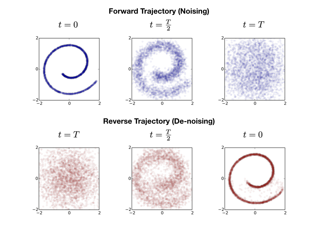Figure 1: adapted after Sohl-Dickstein et al., (2015): shows forward (noising) and reverse (de-noising) diffusion trajectories. Forward gradually adds noise, whereas reverse sequentially removes it, recovering data structure. \(t\) is “time” of diffusion with \(t=T\) corresponding to Gaussian noise (think of it as completed diffusion process) and \(t=0\) - to input/recovered data (diffusion has not started or is “reverted”).

While there are many wonderful tutorials online, I attempt to provide an explanation of the process based on a perhaps obvious intuition, which, at the same time, helped me clear my personal understanding of the subject. Obvious intuition is a term I use to refer to a simple plain language explanation of a concept. While sometimes it can be overly simplified, it is how I would “explain like I am five” (well… I am definitely older than five, and the explanation is a bit more complex too). Detailed mathematical expressions are provided as well, with complexity increasing towards the end.

There are two main goals for this blog series. First, provide an intermediate level explanation without skipping any steps. Often details are omitted because they are either too ‘trivial’ for experts or too ‘hard’ to explain in the bird-eye-view reviews. Second, describe diffusion-related concepts within the same context. Often, I would be referred to different resources to remind myself about VAEs (Variational Autoencoders), for instance. Here, diffusion building blocks are gathered in one place. I do hope these goals are met at least partially.

Among many giants there are two, on whose shoulders the narration stands: the papers by Sohl-Dickstein et al., (2015) and Ho et al., (2020). The first paper draws inspiration from thermodynamics to introduce diffusion models, the second simplifies their training framework and introduces Denoising Diffusion Probabilistic Models (DDPMs), which are the focus in this blog series. While DDPMs are not that hyped on their own, they are fundamental to Latent Diffusion Models (LDM), where they operate in the compressed image space, i.e., so-called latent space, and not in the input image pixel space directly (Rombach et al., 2022). In its turn, a much more ‘famous’ Stable Diffusion model follows the LDM’s latent space setup (Esser et al., 2024: page 4, second 4, paragraph 2).

The Stable Diffusion model consists of three construction blocks: obviously, DDPM (based on a denoising neural network (UNet)), but also a text encoder, and an autoencoder (Perez et al., 2023). Autoencoder performs above-mentioned image compression (Rombach et al., 2022): it reduces original image dimensions and allows for significant computational cost reduction since diffusion is now run in a smaller domain. After diffusion completes, original image dimensions are recovered by a decoder. A text encoder, in its turn, allows for conditioning on a text prompt, which guides reverse diffusion to produce image compositions as requested by the user. Stable Diffusion model without the autoencoder and with no text conditioning (e.g., null text prompt (empty string, for instance) is given, which makes it an unconditional diffusion model) basically corresponds to DDPM applied in the pixel space (keep in mind of course, Stable Diffusion is trained to operate in the latent space). Below, I predominantly focus on Denoising Diffusion Probabilistic Model, and both image compression and conditioning on text are out of scope of this blog series.

I start with a brief introduction (below), where I draw an obvious connection with a physical diffusion process. We then proceed with Statistical Foundations chapter, where latent variables - key hidden factors controlling our data characteristics - are introduced and searched for using Variational Inference (VI)\(^*\). Within the VI framework, we optimize for approximate probabilities, which statistically relate data and latents, thus enabling data generation/reconstruction by generative models, discussed in the following section. We discuss VAEs, and through Hierarchical VAEs (HVAEs) work our way up to Markovian HVAEs, which are a close DDPM sibling with encoders and decoders operating on latent hierarchies with dependence on the previous latent level only. With all the building blocks described, we proceed with DDPMs. First, we focus on a single forward (noising) and reverse (de-noising) diffusion operators. We then formulate an objective function to optimize the reverse process as a whole. Finally, we condense the objective function to a ‘simple’ noise estimation problem. Brief summary of the series follows. Notations are provided in Appendix A.

\(^*\)as of February 2025 this is when the published material ends.

Let me introduce someone special before proceeding - meet ink-tolerant Gold Fish Emma. She greatly helps us in the ‘Basic Intuition’ section, where without her we would lose track of the potential reverse trajectories. Emma also accompanies us throughout the blog series, asks for clarifications, where necessary and, overall, holds me accountable. Regarding her presence in a tank with ink - no worries, she is ink tolerant and in fact enjoys changing colors temporarily. Also the diffusion processes we consider are slow, which means the water temperature is very comfortable for her (see the relation between diffusion speed and temperature below).

Figure with no number: an artistic portrait of ink-tolerant Gold Fish Emma using DALL⋅E 2. No real photographs are used for the protection of privacy.

Introduction

The importance of diffusion models comes from their ability to overcome limitations of GANs and VAEs. In particular, generation process in the latter two models may regress towards the “average” image/sample of the dataset (so-called mode collapse) resulting in a low variety of produced outputs (IntroToDeepLearning.com). Sohl-Dickstein et al., (2015) formulate advantages of diffusion models as: “Most existing density estimation techniques must sacrifice modeling power in order to stay tractable and efficient,” while diffusion models, given the number of steps is made large, can “learn a fit to any data distribution” and remain “tractable to train, exactly sample from, and evaluate.” My obvious intuition is as follows: it can be easier to approximate a complex data distribution by a set of small steps as opposed to learning a complex yet single approximator.

Basic Intuition

The approach is proposed by Sohl-Dickstein et al., (2015) and referred to as Diffusion Probabilistic Models. The authors propose a two-step process: first systematically and slowly destroying structure in input data, then learning a reverse process to restore this structure. The method uses a Markov chain, which, among many other applications, models Brownian motion. For Brownian motion (and Markov chains), the future state of the particle (event) depends only on the current state of the event, not on the history of previous states. A change of state is controlled by transition probabilities, which can be described by Gaussians. Brownian motion is responsible for the phenomenon of diffusion (University of Chicago Statistics Course).

The systematic and slow process of destroying structure in data, referred to as the forward diffusion process, corresponds to a set of Gaussian transitions describing Brownian motion. The forward process is a Markov chain that gradually adds Gaussian noise to the data (Ho et al., 2020). To continue the obvious analogy, think of the input image as initial concentration of paint or ink. With time proceeding, initial concentration (by the means of Brownian motion) evens out into a uniform distribution of pixels corresponding to a normal distribution.

A single Brownian step of the forward process can be mathematically described as a Gaussian transition (Ho et al., 2020), where the result depends on the previous state of Brownian motion. In other words, obviously, how ink is distributed at a given diffusion time depends on how it was distributed a time step before. The distribution is described by a Gaussian function with a mean depending on a previous step. Notice, it only depends on a previous time step and does not use information from previous steps (Markov chain property). So, it is not like we “just” add some random noise to images: we model physical diffusion process by mathematically reproducing a set of Brownian motion steps. Well… We end up noising the images, but using Gaussian transitions, each of which takes a previous noisy version as an input.

If we can reverse the above process, we can generate an image from a Gaussian noise input (Lilian Weng blog). Here, the obvious analogy corresponds to the recovery of the initial ink concentration after it has diluted in water over time. How would we construct such a reverse process? If forward diffusion is happening “slowly” (an obvious analogy would be ink diffusion in relatively cold water as opposed to boiling) or Brownian jumps are small or, equivalently, you do not noise an image too much at each step, then you could backtrack or revert a Brownian step and find out which previous state (less noisy image) caused current state (noisier image). More formally, if a variance is small enough, reverse diffusion process has the identical functional form of the forward process (Sohl-Dickstein et al., 2015). This means that the reverse process of recovering data structure corresponds to Brownian motion with a Gaussian transition probability as well.

So, we need to revert a Brownian step… Unfortunately, unlike the forward case, in which we add noise to a previous less noisy image, this is, in general, an intractable problem. Recovering a previous state of the system based on the current observation is an ill-posed problem with multiple solutions: multiple Brownian steps from multiple previous states could all produce the same state of the system at an observed diffusion time of \(t\) (see schematic in Figure 2, where alongside a true particle distribution at \(t-1\), Brownian steps from two other hypothetical concentrations can result in the distribution at time \(t\)).

This challenge has two aspects: first, the stochasticity of transitions, each of which has a certain probability and hence the uncertainty. Second, the systematic direction of denoising: if we don’t know what is behind noise, how would we know the correct reverse transition? However, if a noise-free image, on which our forward diffusion has operated, is known, then there is a closed-form expression for a reverse Brownian step (see Ho et al., 2020, equation 7). While, in general, reverting diffusion steps is intractable: there are just too many system states you could arrive at the current step from (see Croitoru et al., 2023, page 4, second to last paragraph), - when you know the original input, you know what noising trajectory took place and hence we get a particular reverse Brownian jump. Once again, the reverse process becomes tractable when conditioned on input images (Ho et al., 2020).

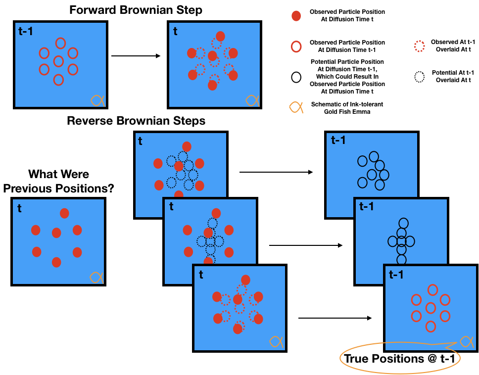Figure 2: A schematic showing reverse process intractability: multiple previous steps could result in the current observed state of diffusion at time \(t\). Goldfish Emma sees the forward noising process of a particular input image. Thus, Emma can help us find the reverse Brownian jump, which, amongst many other possible system states at \(t-1\), corresponds to a given image she saw during noising. In this sense, if we check with her, we can collapse the manifold of all reverse diffusion steps to the one, which takes the place when we noise our given input image. Formally, “forward process posteriors… are tractable when conditioned on” input data (Ho et al., 2020; think of forward process posteriors as reverse diffusion steps). Emma uses strict mathematical logic when helping us to choose correct reverse Brownian steps, which I share further down the text.

Interestingly enough, we have just briefly described how diffusion models are trained under a ‘simple’ de-noising objective. We have all the ingredients to train a de-noising neural network and then predict images from noise. We know the form of the forward noising process and can create de-noised training labels from the reverse process, conditioned on input images (Luo, 2022). Concisely, to tackle general reverse process intractability, you train on a tractable reverse process, conditioned on input data, and learn to approximate the distribution of input images. The trained network is then applied in a number of steps to revert the diffusion process and create an image from noise: step by step we reverse the noising process until a Swiss-roll image shows up. You now have sampled an image from the learnt distribution.

I hope this high-level sketch is illustrative and suggest to proceed with the Statistical Foundations chapter, where we start formulating diffusion model building blocks with more mathematical rigor.